
The Situation
At some stage in the manufacturing process, just about every manufacturing plant in the world makes and/or packs raw materials and finished product. These could be solids, granules, powers, slurrys, liquids and/or gases. They are repeatedly, filled or dispensed into or from containers or vessels to a defined tolerance specification.
The measurement and control of these raw material and finished product events happens many hundreds of thousands or millions of times a year. Even a very small error in every dispensing or filling event, adds up to a very large number at the end of 365 days.
The Objectives
The objective is to stay within specific tolerances to ensure:
• Minimal waste of raw material or finished product is achieved (cost containment)
• Finished product quality and regulatory & safety requirements are met (Adherence to standards)
• Finished product performance consistently meets customer expectations (sales growth)
The Challenges
It might seem a simple task, however there is a lot going on when a product is being filled or dispensed, “THINGS” most people do not know or have not thought deeply about.
Automating these manufacturing events requires 3 integrated elements that all work together to form a CONTROL LOOP:
1. Measurement device, such as an industrial scale
2. Control device, such as a PLC
3. Suitable final control device, such as a screw feeder, vibratory feeder, ball valve, pump etc.
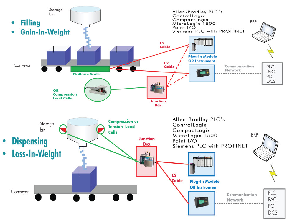
The control loop measures the weight of the raw material or finished product as it enters (gain-in–weight) or leaves (loss-in-weight) the container or vessel that is resting on the scale. The weight information is updated and communicated to the controller throughout the fill or dispense cycle.
The PLC reads this information and compares every update it gets from the scale to a set-point (target weight) it has been instructed to use for this specific event. The PLC is in control of the whole event: starting the event by telling the final control device to open once all “pre-conditions” have been met for the cycle e.g. scale is at zero, scale is not in motion, enough material is available to reach the set-point and others as required. Once the set-point is reached, the PLC instructs the final control device to close and shut off the cycle. Getting the control loop right is just half of the story and the challenge.
Now let’s look at the other half of the challenge. The CONTROL LOOP interacts with the PROCESS. Between the CONTROL LOOP and the PROCESS there are “4 HIDDEN THINGS” going on that contribute to and add up to over or under filling or dispensing errors. They are:
1. IN FLIGHT MATERIAL: This is the amount (weight) of material that has passed through the final control device and cannot be stopped, but has not yet reached the scale and been measured. This contributes to an over fill or dispense error.
2. MEASUREMENT DELAY: There is a time delay between the scale reading the amount (weight) of material currently on it; and what the PLC believes is on the scale from the last update when it decided whether to tell the final control device to stay open or to close. This time delay represents an amount of material (weight) and contributes to overfill or dispense error.
3. FINAL CONTROL ELEMENT LET THROUGH: Unfortunately, there are no final control devices that can “instantaneously” stop material feeding when they receive the instruction to shut off from the PLC. All take some time to close off the fill or dispense cycle and again this time required represents an amount of material (weight). This contributes to an over fill or dispense error.
4. KINETIC ENERGY IMPACT: Finally there is the “force” of the material that impacting the scale that occurs in addition to the actual “weight” of the material that the scales reads in a filling event. This force is reads as “weight” that does not actually exist. This contributes to an under fill error. It does not contribute to dispense errors.
Sadly, it does not stop there. If all of these errors were constant in every fill or dispense cycle, then we could simply calculate them, add them up and compensate for them in every feed. In the real world, the “THING” is that PROCESS conditions do not stay constant. By that we mean that the rate at which materials “FLOW” can change over a period of time (mins or hours, etc) or even from one cycle to the next, based on many variables such as changes in head pressure, viscosity, density, humidity etc.
So there we have it. Changes in process conditions will influence flow rates, which in turn will adjust the amount of “over or under” fill or dispense error that each of the above “4 THINGS” contribute.
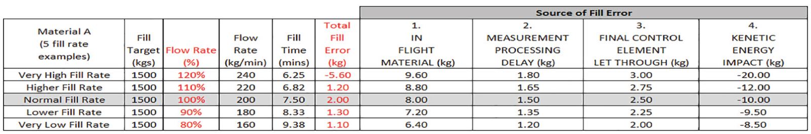
The table below illustrates 5 fill cycles where the filling rate has been increased and decreased in steps of 10%. The grey line shows the optimum fill rate at 100%. One might expect the overfeed error to steadily increase as the fill rate is increased from 80% to 120%. However that is often not the case. Notice that at 110% the error decreased to 1.2kg from 2kg at 100%, and then at 120% it goes negative to -5.6kg. Why? Because the first 3 sources of errors all contribute over feed (+) errors, the 4th contributes an under feed (-) error. As the fill rate increases the Kinetic Energy can reach a point where its force “phantom weight value” surpasses the sum of the first 3 sources of errors. This creates a non-linear acceleration/deceleration in the error curve in most filling application. Again this is not the case in dispensing applications because no Kinetic Energy for is in play.
The Solution
So what to do? There are 3 potential approaches. We will discuss each of these options, in depth. They encompass:
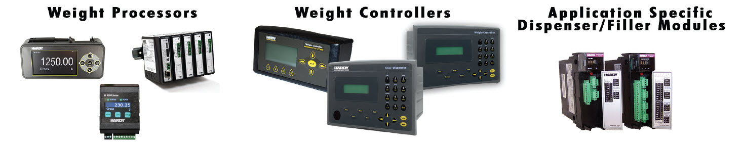
• Controlling process changes with weight processing
• Constricting and adapting to process changes with weight controllers
• Predicting and adapting to process changes with dispenser/fillers
Approach #1: Controlling Process Changes
This approach is usually only deployed when filling or dispensing slurries, liquids or gasses. Why? With these forms of material we can “eliminate” the effect of gravity, by controlling the pressure inside the sealed container or vessel that we are feeding the material from.
Think of a 30 foot high, 10 foot wide vessel holding a liquid with the dispensing valve located at the bottom of the vessel. When the vessel is full (30 foot column of liquid) the head pressure on the valve is at its highest and material will flow at its faster rate. When the vessel is a third full, the head pressure will be significantly reduced and material will flow at a slower rate – affecting the 4 THINGS mentioned above. In fact, every time material is taken from the vessel the height of the column of material gets lower, which in turn reduces the head pressure and the 4 THINGS change slightly.
What’s the control engineer's answer to solving this problem? Use a sealed vessel that can be pressurized and control and hold the pressure in the vessel at a constant level. A few examples of this approach would be: Color Kitchen batch applications producing inks or dyes; and multi-head rotary fillers, filling juices, oils etc.
The benefit (PRO) of this approach is clear, by eliminating the process variable created by gravity we eliminate changes in the 4 THINGS.
The downsides (CONs) are:
1. That the cost to implement, automate and control the pressurized vessel can be high.
2. This approach does not work for all materials e.g. aggregates, granules and powders.
Approach #2: Constricting and adapting to process changes
Now let’s take a look at another widely used approach. In this case the control engineers are aware that the material flow rates are going to vary for multiple reasons – material flow characteristics changing because of moisture, temperature etc. and also head pressure. So in this case they decide to “minimize” the process changes and therefore the errors that would be created by the “4 THINGS”.
How? They choose to control the feed rate (flow rate) of the material during each feed or filling cycle. They do this by using two pumps or two valves depending of the material types they are dealing with. This type of approach is called multi-speed feed control. As an example: consider feeding material from the same 30 foot vessel mentioned above, but this time we are not going to seal it and pressurize it. Instead we are going to have 2 outlets at the bottom on the tank – the first will be a 6 inch pipe with an on/off slide gate and the second a 1 inch pipe with an on/off slide gate.
When the feed starts both vales are opened (effectively 7 inches of flow rate is feeding material) this is called the “fast feed” stage. As the feed is approaching the set point and gets to within say 5% of the target, the control system shuts of the 6-inch slide gate. This effectively slows (constricts) the flow rate down to 1/7th of the fast feed rate – the feed is now in what is termed “slow feed” stage. What just happened? Constricting the flow effectively reduced all process variation to 1/7th and the impact of all errors created by the “4 THINGS” to 1/7th. In this case there will still be an error but it will be greatly reduced. Whatever the error was can be recorded, and a portion of it (say 50%) used as feedback to adjust a pre-act value that triggers the “slow feed” stage to stop just before the feed target is reached. Or after if the Kinetic Energy in the “slow feed” stage exceeds the other “3 THINGS”. An easy way to think of what was done is to imagine you are “throttling the process changes and errors almost to death” to minimize any variations caused by moisture, temperature, head pressure etc.
The benefit (PROs) of this is approach is clear:
1. It “minimizes” errors from the “4 THINGS”
2. This approach will work for ALL materials types
The downsides (CONs) are:
1. The cost to implement, automate, control and clean multiple feeding outlets can be high
2. Slowing the process flow rate in every feed “steals time” from production – filling line and batch cycle times become longer. This reduces the number of bottles that could be filled in an hour or the number of batches that can be produced in an hour.
Approach #3: Predicting and Adapting to Process Changes
This approach was developed more recently and was motivated by:
1. The high cost of implement and maintaining the control systems or loops
2. The need to maximize filling rates and batch cycle times in high performance manufacturing supply chains
3. The desire to simultaneously minimize feeds errors as much as possible. Remember the Holy Grail of feeding materials is to feed the exact amount of material, in the minimum amount of time, every time!
So is this possible? Well this time instead of “controlling or constricting” we are going to try to “measure and predict” what has changed since the feed started, then adapt for the change. Let me explain where this idea came from by switching gears completely for a moment.
Think about a gunner on a ship back in WWII trying to shoot down an enemy aircraft. The aircraft is a moving target, the shell the gunner is about to fire will take some time to reach the aircraft – so the gunner tries to anticipate where the aircraft will be when the shell gets to it by firing slightly in front.
But the planes air speed could be changing, wind speed and direction both could change. The bottom line is that it is challenging for the gunner. This challenge is what motivated the invention of the missile, which is fired in the general direction of the target, but tracks any changes in the targets position down to the last second before impact. I think you get the picture.
A similar thing is going on during a material feed. Process conditions are changing the flow rate. Now we don’t have the luxury of a missile, but we have one advantage over the gunner in that we can use the weight controller to predict and track down and adapt to any process changes to the last second, and that one thing is “FLOW RATE”. By measuring the weight and flow rate simultaneously we can adjust and “dial in” pre-act value throughout the feed, without having to control or constrict the flow rate.
By monitoring flow rate we can maintain a fast flow rate all the way through the feed down to the last second before impact, in other words all the way to the set point (target weight).
The benefits (PROs) of this are approach is clear:
1. We don’t have to worry about the process variability and potential errors from the “4 THINGS”
2. This approach will work for all materials types
3. That the cost to implement, automate, control and clean in most cases can be reduced to one multispeed valve/gate and slowing the process flow rate in every feed is not required in most cases so “stealing time” from production does not happen. Filling line and batch cycle times become shorter.
This increases the number of bottles that could be filled in an hour or the number of batches that can be produced in an hour.
The downsides (CONs) are:
1. Feed upsets e.g. wildly varying flow rate can still create feed errors. However, this approach takes us much closer to the “Holy Grail”.
If you are wondering how often each approach is deployed in the real world? A best guess (estimate) based on experience would be: Approach #1 in approximately 10% of applications; Approach #2 in approximately 70%; Approach #3 in approximately 20%.
We believe that as more and more control engineers engage in the use of advanced control methods, and discover and deploy the third approach that it will eventually reach about 50% of future applications.
How Hardy improves OEE with Faster Installations, Calibrations and Diagnostics
Hardy has the expertise and innovative solutions to assist your team in reducing cost and increasing yield, while limiting downtime and achieving improved Overall Equipment Effectiveness (OEE). Hardy products are easy to install, configure, commission, operate and maintain. They are safer and save you time, money, raw materials and/or finished product. By implementing these simple built-in Hardy process weighing tools, you can increase your Operational Equipment Efficiency (OEE), safety, and reliability today. Red the application note here.
The above article was written by Rodger Jeffery, who has been with Hardy Process Solutions for 11 years and in the industry for 40 plus years. He has solved simple and complex weighing related problems in many manufacturing industries and has installed thousands of INDUSTRIAL WEIGHING solutions across the globe.

To learn more about how Hardy Process can greatly
improve your process weighing application, reach out to us today!
csr@finnandconway.com
(708) 599-0103